

Concept
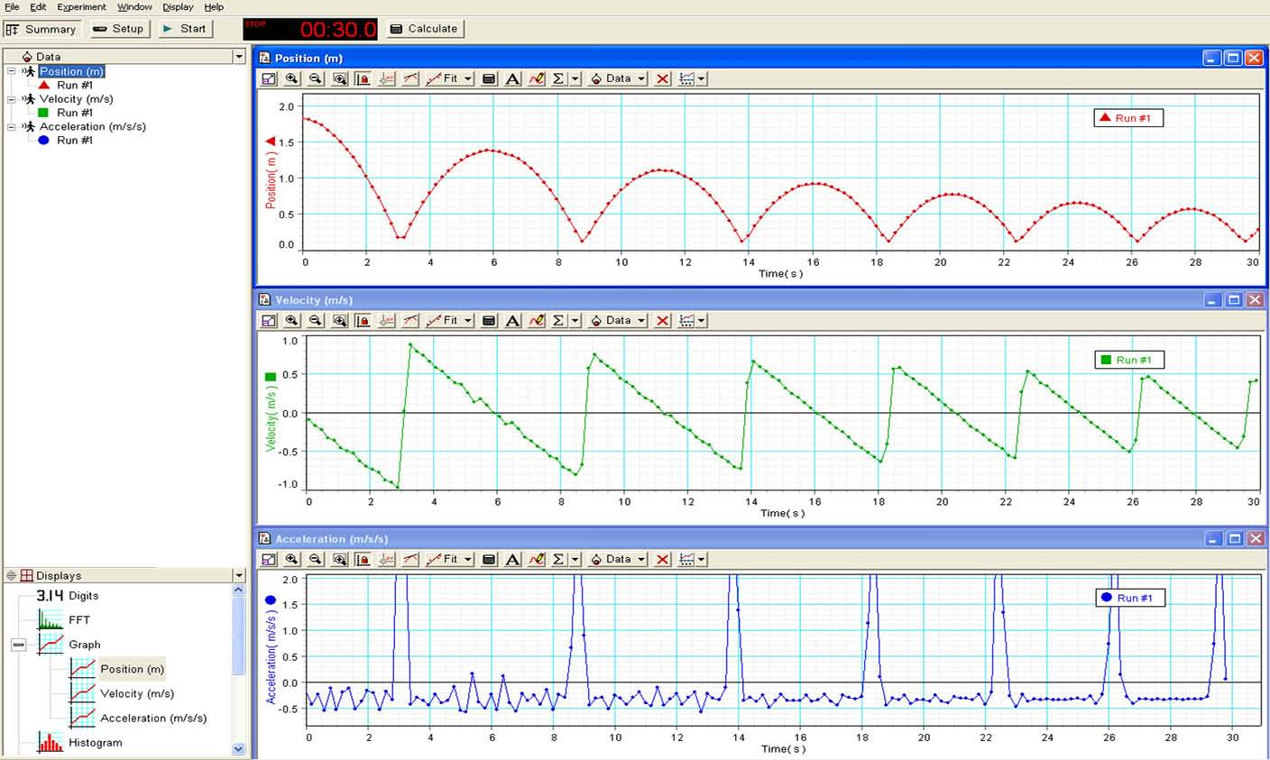
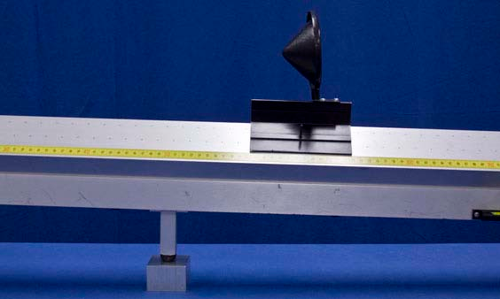
Challenge your students to sketch graphs of $x(t)$, $v(t)$ and $a(t)$ for a bouncing ball. Then, show them the real time graphs for the qualitatively similar case of a glider bouncing on an inclined track.
Talking points: Between bounces, the acceleration reads $−0.3 \text{m}/\text{s}^2$ (the noise about this value smoothes out with time). This value of acceleration can be confirmed by examining the slope of the corresponding $v(t)$ graph. Acceleration between the bounces can also be checked using $g \sin(\theta) = (− 9.8 \text{m/s}^2 )$ the block is 3.4cm and the length of the support base is 100cm. During a bounce, the peak acceleration can be determined from the slope of the $v(t)$ graph. For the first bounce this gives $\frac{1.9 \text{m/s}}{0.3\text{s}} = 6\text{m/s}$ and thus is on order of one $g$.
Friction between the glider and track, thermal dissipation in the rubber bumper, and air resistance, all act to reduce the bounce amplitude.
Procedure
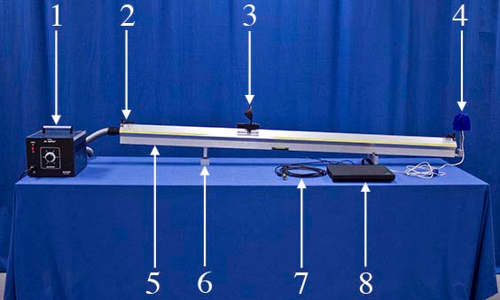
- Verify that the Pasco Motion Sensor is connected to the laptop and that the DataStudio software suite is open to the “Inclined Air Track” activity. Turn on the air supply.
- Press the “Start” button on the screen to start the 5-second countdown to data collection. (If the “Start” button is grayed out, unplug the motion sensor’s USB cable and plug it back into the computer.)
- Quickly position the glider near the top of the air track incline and release it at about the same time that data collection begins.
- Notice that the glider’s position, velocity and acceleration are plotted in real-time for 30 seconds.
- To erase all collected data and repeat the demonstration, click on the “Experiment” menu and select “Delete All Data Runs.”
Equipment
- Air Supply
- (2) Bumpers
- Glider with Sonic Reflector
- Pasco Motion Sensor
- Air Track
- Aluminum Block (3.4cm)
- VGA Extension Cable
- Laptop with Pasco DataStudio